| Issue |
Ann. For. Sci.
Volume 66, Number 8, December 2009
|
|
|---|---|---|
| Article Number | 804 | |
| Number of page(s) | 9 | |
| DOI | https://doi.org/10.1051/forest/2009071 | |
| Published online | 25 November 2009 | |
Original article
Measuring wood density by means of X-ray computer tomography
Mesure de la densité du bois par tomographie à rayons X
INRA, UMR1092 LERFoB, 54280 Champenoux, France AgroParisTech, UMR1092 LERFoB,
54000 Nancy,
France
* Corresponding author: This email address is being protected from spambots. You need JavaScript enabled to view it.
Received:
26
January
2009
Accepted:
21
April
2009
Abstract
• Wood density is a characteristic of major interest. Usually, it is used as an indicator of wood quality; however, in the context of global change, it is increasingly used for biomass and carbon storage estimations. X-ray computer tomography is a method which enables quick estimates of wood density after applying a calibration procedure.
• A review of the literature is presented in this article. Most of the previous studies have been performed in the 80’s or at the beginning of the 90’s.
• In this study, the relationship between wood density and Hounsfield numbers was investigated using a recent medical scanner. A linear relationship was fitted using a calibration data set which consisted in tropical wood samples representing a large range of densities ranging between 133 and 1319 kg m−3, and then validated using an independent data set (mainly temperate tree species). The fitted relationships were very strong (R2 > 0.999), whichever the tested scanner settings, with slight but significant effects of the current voltage and reconstruction filters. The RMSE values computed from the validation data set ranged between 5.4 and 7.7 kg m−3 for densities ranging between 364 and 821 kg m−3.
• In conclusion, this method of calibration enables the use of a medical scanner to obtain maps of wood density, in a fast and non destructive way, and with a very good accuracy. Very interesting perspectives are opened regarding biomass distribution within trees.
Résumé
• La densité du bois est une caractéristique d’intérêt majeur. Généralement, elle est utilisée comme un indicateur de la qualité du bois ; cependant, dans le contexte du changement global, elle est de plus en plus utilisée pour des estimations de biomasse et de stockage de carbone. La tomographie à rayons X est une méthode permettant des estimations rapides de la densité du bois moyennant une procédure de calibration.
• Une revue de la littérature sur le sujet est présentée dans cet article. La plupart des études précédentes ont été réalisées dans les années 80 ou au début des années 90.
• Dans cette étude, la relation entre la densité du bois et les nombres Hounsfield a été étudiée en utilisant un scanner médical récent. Une relation linéaire a été ajustée sur un jeu de données de calibration constitué d’échantillons de bois tropicaux représentant une large gamme de densités allant de 133 à 1319 kg m−3, et validée sur un jeu de données indépendant (principalement des essences tempérées). Les relations ajustées étaient très fortes (R2 > 0.999) quels que soient les réglages utilisés pour le scanner, avec des effets légers mais significatifs de la tension d’accélération et des filtres de reconstruction. Les valeurs des RMSE calculées à partir de l’échantillon de validation sont comprises entre 5.4 et 7.7 kg m−3 pour des densités allant de 364 à 821 kg m−3.
• En conclusion, la méthode de calibration proposée permet l’utilisation d’un scanner médical pour obtenir de façon rapide et non destructive des cartes de densité du bois avec une très bonne précision. Des perspectives très intéressantes sont ouvertes concernant la répartition de la biomasse dans les arbres.
Key words: wood density / X-ray computer tomography / CT / Hounsfield numbers / calibration
Mots clés : densité du bois / tomographie à rayons X / CT / nombres Hounsfield / calibration
© INRA, EDP Sciences, 2009
1. INTRODUCTION
Wood density is a characteristic of major interest in trees. For industrial uses (e.g. wood constructions, pulp and paper), wood density is a determinant of the quality as it is highly correlated with the mechanical and physical properties of wood (e.g. strength, shrinkage). In the context of global change, there is a strong demand for the estimation of forest biomass with two main objectives: the production of energy from the available forest resource (wood is the first sustainable source of energy in the world and its density is not only important for estimating the amount of biomass but it is also correlated with its calorific value), and the assessment of carbon storage in standing trees and wood products. Biomass estimations can be obtained by direct models (Zianis et al., 2005) or by indirect approaches combining volume and wood density estimations in trees (Vallet, 2005). Some other studies, performed at a finer scale, investigate the link between intra-ring wood density and anatomical characteristics (e.g. Rathgeber et al., 2006). Moreover, the moisture content distribution in wood, which is important both for industrial (e.g. shrinkage) and physiological aspects (e.g. sap and water flows), can be assessed through the analysis of density variations during drying (Fromm et al., 2001).
X-ray computer tomography (CT) is a powerful methodology which enables to compute 3D maps of objects based on X-ray attenuation. The linear attenuation value μvoxel of each voxel belonging to the object is computed from X-ray projections through the object, in several directions. CT scanners were first developed for medical applications and are now largely used in the field of medicine. More recently, they started to be used for wood applications. The first uses of CT scanners in this area were done in the 80’s with the internal defect detection as a main objective (among others: Benson-Cooper et al., 1982; Funt, 1985). The X-ray attenuation depends on the atomic composition of the studied material and on the X-ray energy (Mull, 1984; Lindgren, 1991b). To enable comparisons between images obtained with different scanners (operating at different X-ray energies, for instance), a normalised unit was defined. The Hounsfield numbers or indices (H), or CT numbers, are normalised against the X-ray attenuation of water as follows:  Each manufacturer of commercial scanners provides a calibration procedure, generally using a water filled phantom, which must be launched periodically to ensure that H = 0 in water and H = − 1000 in air whatever the X-ray energy used. Nevertheless, the Hounsfield numbers measured on air were shown to depend on the scanner model and settings and on the scan date, even for recently manufactured devices (Parr et al., 2004). Moreover, for low energies, differences in atomic composition may lead to differences in X-ray attenuation even for objects of the same density (Macedo et al., 2002). Since the atomic composition of wood may differ strongly from the material used for CT calibration, it appears important to calibrate the device specifically for the estimation of wood density ρ.
A rough rule of calibration is:  The accuracy of this calibration rule is about of 10%, which is considered adequate for rapid feasibility studies (Davis and Wells, 1992). More accurate rules can be found in the literature (Benson-Cooper et al., 1982; Davis and Wells, 1992; Hattori and Kanagawa, 1985; Lindgren, 1991b; Mull, 1984; Taylor, 2006). From the literature, the relationship between ρ and H is linear and the adjusted equations are of the form:
  Most of these equations were obtained with relatively old scanners which differ slightly from the currently available models.
This study investigates the relationship between wood density and Hounsfield numbers, for a multi-slice CT scanner (GE BrightSpeed Excel acquired in 2007), for a large range of densities obtained by analysing samples of both temperate and tropical tree species, and considering several filters in the reconstruction process. In particular, we assessed the linear shape of the relationship for extreme wood densities. Non-linear relationships were found by extending the range of densities with other materials of high densities like graphite or titanium (Mull, 1984; Saw et al., 2005). In the discussion section, our calibration equations were compared with the ones found in the literature.
2. MATERIALS AND METHODS
Two series of wood samples were used to produce calibration and validation data sets, respectively. The sample used to calibrate the relationship between wood density and Hounsfield numbers consisted in 16 cubes (of about 3 × 3 × 3 cm) of tropical tree species selected in order to represent a large range of density values. In this way, we attempted to reduce as much as possible the further use of the calibrated relationship in extrapolation. The validation sample consisted in 21 cubes (of about 2 × 2 × 2 cm) of mainly temperate tree species which are of major interest in France, with 3 cubes per species.
Before starting the experiment, the wood samples were stored in the scanner room until their weight was stabilised. The wood samples were weighted with a laboratory balance and measured in the three directions with a vernier calliper in order to estimate their air-dried density (i.e. at about 12% moisture content) by dividing their mass by their volume. The relative error of measurement of the density obtained by the gravimetric method can be computed as followed:  with ρ the density, m the mass of the cube, d1, d2 and d3 the three dimensions which were measured for computing the volume of the cube, Δρ the error associated to the density
computation, and Δm, Δd1, Δd2 and Δd3 the errors of measurements associated to the balance and vernier calliper. In our case, Δm = 0.0001 g and Δd1 = Δd2 = Δd3 = 0.01 mm. Hence, the mean errors of measurement were of about 0.7 kg m−3 and 0.9 kg m−3 for the cubes of the calibration and validation samples, respectively. Characteristics of the wood samples are presented in Tables I and II.
with ρ the density, m the mass of the cube, d1, d2 and d3 the three dimensions which were measured for computing the volume of the cube, Δρ the error associated to the density
computation, and Δm, Δd1, Δd2 and Δd3 the errors of measurements associated to the balance and vernier calliper. In our case, Δm = 0.0001 g and Δd1 = Δd2 = Δd3 = 0.01 mm. Hence, the mean errors of measurement were of about 0.7 kg m−3 and 0.9 kg m−3 for the cubes of the calibration and validation samples, respectively. Characteristics of the wood samples are presented in Tables I and II.
Characteristics of the wood samples used for calibrating the relationship between wood density and Hounsfield numbers.
Characteristics of the wood samples used for validating the relationship between wood density and Hounsfield numbers.
Then, the same day, at the same moisture content, the wood samples were X-rayed in a medical CT scanner GE BrightSpeed Excel. Figure 1 shows the arrangement of the cubes into the scanner, with the X-ray beam perpendicular to the grain. The reconstructed CT images are 512 × 512 pixels. The fields of view were 180 mm and 160 mm for calibration and validation samples, respectively. The slice thickness was set to 1 cm which was the maximum authorised value. Hence, the voxel sizes were 0.35 × 0.35 × 10 mm3 and 0.31 × 0.31 × 10 mm3, respectively. Several scanner settings for the acquisition parameters were used: 80 and 120 kVp; 50, 80 and 200 mA; and all seven reconstruction filters available, respectively identified as Bone, Bone+, Detail, Edge, Lung, Soft, and Standard1. This resulted in 2 × 3 × 7 = 42 tested combinations of settings.
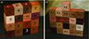 |
Figure 1 Arrangement into the scanner of the wood samples from the calibration (a) and validation (b) data sets. |
For each cube in each CT image, the mean and standard deviation of Hounsfield numbers were computed. In order to avoid edge effects, a central square area of interest was designated for each cube representing 81% (5929 pixels) and 79% (3600 pixels) of the total cube transverse area for calibration and validation samples, respectively (and corresponding to 27% and 38% of the total cube volume, respectively, due to the slice thickness of 1 cm in the grain direction). Since the means of Hounsfield numbers were computed on partial volumes within the cubes, it was assumed that – at the studied scale – the cube density was homogeneous enough in the grain direction to allow the comparison with measured gravimetric densities of the whole volumes.
The statistical analysis was performed using the R software (Crawley, 2007).
3. RESULTS
3.1. Scanner setting and reconstruction filter effects on Hounsfield numbers
Raising the current voltage from 80 to 120 kVp significantly increased the mean of measured Hounsfield numbers by around 10 units (Fig. 2). The current intensity and the reconstruction filter (except Lung and with less importance Soft and Standard) did not have noticeable effect on the mean values. These results shown in Figure 2 were confirmed statistically by ANOVA.
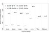 |
Figure 2 Mean of Hounsfield numbers computed from the calibration data set for several combinations of the scanner settings. |
On the other hand, the range of variation of the Hounsfield numbers in a CT image (here estimated by averaging the standard deviations of the 16 cubes) depended mainly on the reconstruction filter used (Fig. 3). This effect was observable with the naked eye on the images (Fig. 4), which seemed more or less smoothed or noised, depending on the filter used for the reconstruction. On a scale ranging from low to high smoothing effect, the filters may be classified as is: Lung, Bone+, Edge, Bone, Detail, Standard, and Soft.
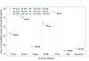 |
Figure 3 Mean of Hounsfield number standard deviations computed from the calibration data set for several combinations of the scanner settings. |
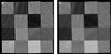 |
Figure 4 CT images obtained from the calibration wood samples at 120 kVp and 50 mA with two different reconstruction filters; Lung (a) and Soft (b). |
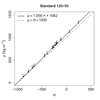 |
Figure 5 Linear regression between Hounsfield numbers H and wood density ρ, adjusted using the calibration data set, for the Standard reconstruction filter, 120 kVp and 50 mA. |
3.2. Calibration of the relationship between wooddensity and Hounsfield numbers
A regression line was adjusted for each of the 42 combinations of scanner settings. As an example, Figure 5 shows the regression line which was adjusted for 120 kVp, 50 mA and the Standard reconstruction filter. For comparison purposes, the rough calibration rule consisting in adding an offset of 1000 to the Hounsfield numbers was presented on the same plot. The residuals of the regression are presented in Figure 6. Depending on the scanner settings, the regression intercepts ranged between 1043 and 1075, and the slopes ranged between 1.027 and 1.065.
R2 values for the 42 calibration equations ranged between 0.9993 and 0.9998, whereas the RMSE values ranged between 4.5 and 8.0 kg m−3 (Fig.7). It appeared that RMSE values were systematically lower for 120 than for 80 kVp, and that the Lung reconstruction filter showed the highest RMSE values.
Cube #1 from the calibration sample (Brosimum guianense) showed the highest residuals in absolute values in comparison with the other cubes, with in addition strong differences between the current voltage settings (overestimations ranging between 21 and 24 kg m−3 and between 13 and 16 kg m−3, for 80 and 120 kVp, respectively). When cube #1 was removed from the analysis, the R2 increased ranging between 0.9997 and 1, and the RMSE values decreased ranging between 2.6 and 4.9 kg m−3. In the following, we decided to keep cube #1 in the analyses.
A statistical model was adjusted to assess the effects of the scanner settings (reconstruction filters, current voltage and intensity) on the relationship between wood density and Hounsfield numbers. The overall form of the model was as follows:  with
α, αfilter, αkVp and αmA the slope parameters, and μ, μfilter, μkVp and μmA the intercept parameters. In this analysis, current voltage and intensity were considered as factors rather than as continuous variables. Estimates and significances of the model parameters are given in Table III. The current intensity was found to be non significant both on the slope and intercept of the regression. There was a significant effect of the current voltage both on the slope and intercept of the model. Some reconstruction filters gave significant different results from the others, these were: Lung and with less importance Soft and Standard filters. The Lung filter showed inverse effects in comparison with the Soft and Standard filters both on slope and intercept values, the estimated parameters being of opposite signs.
with
α, αfilter, αkVp and αmA the slope parameters, and μ, μfilter, μkVp and μmA the intercept parameters. In this analysis, current voltage and intensity were considered as factors rather than as continuous variables. Estimates and significances of the model parameters are given in Table III. The current intensity was found to be non significant both on the slope and intercept of the regression. There was a significant effect of the current voltage both on the slope and intercept of the model. Some reconstruction filters gave significant different results from the others, these were: Lung and with less importance Soft and Standard filters. The Lung filter showed inverse effects in comparison with the Soft and Standard filters both on slope and intercept values, the estimated parameters being of opposite signs.
Estimates and significances of the parameters of the model used for testing the effects of different scanner settings on the calibration.
3.3. Validation of the relationship between wooddensity and Hounsfield numbers
The calibrated equations were then used to estimate the densities of the cubes belonging to the validation sample. As an example, Figure 8 shows the estimated densities as a function of the measured densities for 120 kVp, 50 mA and the Standard reconstruction filter. Using the validation data set, the RMSE values ranged between 5.4 and 7.7 kg m−3 (Fig.9), which was very satisfying with respect to the density values. RMSE for validation and calibration data sets were of same order, much lower than the standard deviations of the measured gravimetric densities.
4. DISCUSSION
For each tested scanner setting, the averaged Hounsfield numbers were strongly correlated to wood density (R2 > 0.999). The analysis of the model residuals showed that the linear relationship was adapted.
The highest absolute values of residuals were observed for Brosimum guianense for which density was overestimated by 13 to 24 kg m−3 (i.e. 1.2 to 2.2%), depending on the scanner settings. No noticeable singularity was observed in this wood sample for explaining this discrepancy. The behaviour of this cube was probably due to its chemical composition. In comparison with other cubes, this cube was very sensitive to X-ray energy with clearly better results for 120 kVp than for 80 kVp. It is known (e.g. Macedo et al., 2002) that at low energies, variations in the chemical composition of the material cause variations in the linear attenuation coefficient even for materials having the same density. At high energies, the density influence prevails.
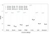 |
Figure 7 RMSE values computed from the calibration data set for several combinations of the scanner settings. |
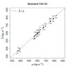 |
Figure 8 Relationship between predicted densities |

A review of the literature about previous calibrations between wood density and Hounsfield numbers is presented in Table IV. All the authors fitted linear models and reported good correlations (R2 > 0.9 in most cases). In our study, a particular effort was made to calibrate the models on a large range of wood densities from 133 to 1319 kg m−3 (air-dried wood). Only the study by Davis and Wells (1992) used such low wood densities around 100 kg m−3. Regarding high wood densities, the maximum used in the literature was around 1100–1150 kg m−3 (Benson-Cooper et al., 1982; Davis and Wells, 1992; Taylor, 2006). We also tested the effects of several combinations of the scanner settings on the calibrations, which was not investigated before. Lindgren (1991a) compared two reconstruction filters (called Detail and Bone) and showed using a water phantom that they were very different in noise (standard deviation of Hounsfield numbers) but not in mean of Hounsfield numbers. We observed similar results applying seven reconstruction filters for the image acquisition of wood samples. As we worked with averaged Hounsfield numbers computed from wood volumes, our results were not affected by these noise differences. Macedo et al. (2002) proposed a completely different approach of calibration, performed directly on the mass attenuation coefficients (i.e. without using Hounsfield numbers which are normally computed from the attenuation coefficients), to estimate wood density with different types of X- and Gamma-ray scanners (but not with a medical one). With this approach, they obtained a R2 value2 of 0.94, similar with R2 values from the literature (Tab. IV). An improvement in comparison with the previous studies (except Macedo et al., 2002) is that we used an independent data set for the statistical validation of our models.
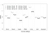 |
Figure 9 RMSE values computed from the validation data set for several combinations of scanner settings. |
Review of the literature about the relationships between wood density and Hounsfield numbers obtained with medical CT scanners.
In most studies dealing with the relationship between wood density and Hounsfield numbers, several trees species were used in order to be representative of a certain range of densities. At the opposite, Espinoza et al. (2005) concentrated on a single species (Acer saccharum Marsh) and chose samples from different tree components (heartwood, sapwood, knots and rot). This parallel approach is interesting even if the chosen methodology may not enable to obtain the best concordance between wood density and Hounsfield number measurements (which could explain the relatively low R2 values obtained, ranging from 0.32 to 0.82). The main objective of this study was to detect valuable parts in trees based on density or moisture content differences by using CT. Depending on the tree components, they found different slopes and intercepts for the regression lines3. In particular, the knots and rot wood showed a noticeably higher slope than the other components. The authors hypothesised that the variations could be due to the difference in the presence and orientation of crystalline structures in the different parts of wood.
Although the results were not presented here, we repeated the same experiment by rotating our cubes by 90°, in a way to scan parallel to grain. No orientation effect was observed on the mean of Hounsfield numbers computed for each cube.
A polychromatic X-ray beam becomes more penetrating as it goes through the matter. This effect, called beam hardening, is considered and corrected in the reconstruction process but one could suspect that the cubes located in the middle of the set of samples (# 6, 7, 10 and 11, see Fig. 1), which received harder X-ray beams than the other cubes, could have a specific behaviour. This effect was checked by repeating the measurements with a new arrangement of the cubes. The cubes #C, I, 1 and 4, which were located at the corners in the first scan were placed in the middle of the square in the new arrangement, the other cubes were placed randomly at the periphery. The regression analysis performed on the new arrangement (not shown) being quite identical to the first ones, beam hardening was regarded as negligible in this study.
A similar work aiming to analyse the effect of moisture content on the calibration equations is in progress. By mixing wood samples with various moisture contents for fitting the regression lines, several authors showed that a single calibration function could be used (Tab. IV). However, according to Lindgren (1991b), woods having the same green density but containing different amounts of water lead to different Hounsfield numbers due to the difference in X-ray absorption coefficients between wood and water. This specific point should be clarified. By repeating the scanning of cubes at various states of moisture content, it would be possible to quantify the effect of moisture changes on the scanner measurements. If the calibration function is not found to be dependent on moisture content (as it can be expected considering previous experiments; Tab. IV, and for high energy X-ray beams; Macedo et al., 2002), it would therefore be possible to measure directly wet and oven-dry wood densities, and then water content maps by subtracting pixel to pixel two CT images of the same wood sample scanned at wet and oven-dry states (after correcting the dimensional changes due to shrinkage).
The methodology described in this paper for calibrating a medical CT scanner in order to measure wood density could be applied to any other CT device.
As a conclusion, this study proved that a medical CT scanner enabled reliable and very accurate estimations of wood density whichever the tree species and the scanner settings used for the image acquisition (R2 > 0.999 and RMSE ranging between 5.4 and 7.7 kg m−3 for wood densities ranging between 364 and 821 kg m−3 in the validation sample). Slight but significant differences were found both on Hounsfield number values and on calibration equations depending on the current voltage (120 kVp gave significantly better results than 80 kVp) and on the reconstruction filter (Lung filter was slightly less accurate than the others). The tested current intensity had no effect on the calibrations, thus we recommend using the minimum tested intensity of 50 mA in order to preserve the X-ray tube. Thus, the CT scanner opens very interesting perspectives for estimations of the biomass distribution within trees, which is a next step of our current work.
Acknowledgments
The authors would like to thank Pierre Gelhaye (INRA Nancy, France) for the preparation of the wood material to be X-rayed and Jacques Beauchene (CIRAD Kourou, FrenchGuyana) for providing the samples for tropical species. Thanks to the Lorraine Region, DRAF and FEDER institutions which financially contributed for the acquisition of the medical CT scanner used in this work.
The reconstruction filters are designed for better working on several parts of human bodies. They are provided “as-is” by the scanner manufacturer without any technical details.
The results of Espinoza et al. (2005) were not reported in Table since they did not work with Hounsfield numbers but with a reduced 256 grey level scale instead.
References
- Benson-Cooper D.M., Knowles R.L., Thomson F.J. and Cown D.J., 1982. Computed tomographic scanning for the detection of defects within logs. FRI Bulletin, Forest Research Institute, New Zealand, 9 p [Google Scholar]
- Crawley M.J., 2007. The R book, John Wiley & Sons, 942 p [Google Scholar]
- Davis J. and Wells P., 1992. Computer tomography measurements on wood. Industrial Metrology 2: 195–218 [CrossRef] [Google Scholar]
- Espinoza G.R., Hern, ez R., Condal A., Verret D. and Beauregard R., 2005. Exploration of the physical properties of internal characteristics of sugar maple logs and relationships with CT images. Wood Fiber Sci. 37: 591–604 [Google Scholar]
- Fromm J.H., Sautter I., Matthies D., Kremer J., Schumacher P. and Ganter C., 2001. Xylem water content and wood density in spruce and oak trees detected by high-resolution computed tomography. Plant Physiol. 127: 416–425 [CrossRef] [PubMed] [Google Scholar]
- Funt B.V., 1985. A computer vision System that analyzes CT-scans of sawlogs. , Proceedings of IEEE Conference on Computer Vision and Pattern Recognition, San Francisco, California, pp. 175–177 [Google Scholar]
- Hattori Y. and Kanagawa Y., 1985. Non-destructive measurement of moisture distribution in wood with a medical X-ray CT scanner I. Accuracy and influencing factors. Mokuzai Gakkaishi 31: 974–980 [Google Scholar]
- Lindgren L.O., 1991. The accuracy of medical CAT-scan images for non-destructive density measurements in small volume elements within solid wood. Wood Sci. Technol. 25: 425–432 [Google Scholar]
- Lindgren L.O., 1991. Medical CAT-scanning: X-ray absorption coefficients, CT-numbers and their relation to wood density. Wood Sci. Technol. 25: 341–349 [Google Scholar]
- Macedo A., Vaz C.M.P., Pereira J.C.D., Naime J.M., Cruvinel P.E. and Crestana S., 2002. Wood density determination by X- and gamma-ray tomography. Holzforschung 56: 535–540 [CrossRef] [Google Scholar]
- Mull R.T., 1984. Mass estimates by computed tomography: physical density from CT numbers. Am. J. Roentgenol. 143: 1101–1104 [Google Scholar]
- Parr D.G., Stoel B.C., Stolk J., Nightingale P.G. and Stockley R.A., 2004. Influence of Calibration on Densitometric Studies of Emphysema Progression Using Computed Tomography. Am. J. Respir. Crit. Care Med. 170: 883–890 [CrossRef] [PubMed] [Google Scholar]
- Rathgeber C.B.K., Decoux V. and Leban J.M., 2006. Linking intra-tree-ring wood density variations and tracheid anatomical characteristics in Douglas fir (Pseudotsuga menziesii (Mirb.) Franco). Ann. For. Sci. 63: 699–706 [CrossRef] [EDP Sciences] [Google Scholar]
- Saw C.B., Loper A., Kom, uri K., Combine T., Huq S. and Scicutella C., 2005. Determination of CT-to-density conversion relationship for image-based treatment planning systems. Med. Dosim. 30: 145–148 [CrossRef] [PubMed] [Google Scholar]
- Taylor A.J., 2006. Wood density determination in Picea sitchensis using computerised tomography: how do density measurements compare with measurements of pilodyn pin penetration? University of Wales, Bangor [Google Scholar]
- Vallet P., 2005. Impact de différentes stratégies sylvicoles sur la fonction “puits de carbone” des peuplements forestiers. Modélisation et simulation à l’échelle de la parcelle. Doctoral thesis, École Nationale du Génie Rural, des Eaux et des Forêts, France. [Google Scholar]
- Zianis D., Muukkonen P., Mäkipää R. and Mencuccini M., 2005. Biomass and stem volume equations for tree species in Europe. Silva Fenn. Monogr. 4: 2–63 [Google Scholar]
All Tables
Characteristics of the wood samples used for calibrating the relationship between wood density and Hounsfield numbers.
Characteristics of the wood samples used for validating the relationship between wood density and Hounsfield numbers.
Estimates and significances of the parameters of the model used for testing the effects of different scanner settings on the calibration.
Review of the literature about the relationships between wood density and Hounsfield numbers obtained with medical CT scanners.
All Figures
|
Figure 1 Arrangement into the scanner of the wood samples from the calibration (a) and validation (b) data sets. |
| In the text | |
|
Figure 2 Mean of Hounsfield numbers computed from the calibration data set for several combinations of the scanner settings. |
| In the text | |
|
Figure 3 Mean of Hounsfield number standard deviations computed from the calibration data set for several combinations of the scanner settings. |
| In the text | |
|
Figure 4 CT images obtained from the calibration wood samples at 120 kVp and 50 mA with two different reconstruction filters; Lung (a) and Soft (b). |
| In the text | |
|
Figure 5 Linear regression between Hounsfield numbers H and wood density ρ, adjusted using the calibration data set, for the Standard reconstruction filter, 120 kVp and 50 mA. |
| In the text | |
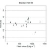 |
Figure 6 Residuals of the regression presented in Figure 5. |
| In the text | |
|
Figure 7 RMSE values computed from the calibration data set for several combinations of the scanner settings. |
| In the text | |
|
Figure 8 Relationship between predicted densities |
| In the text | |
|
Figure 9 RMSE values computed from the validation data set for several combinations of scanner settings. |
| In the text | |