| Issue |
Ann. For. Sci.
Volume 66, Number 6, September 2009
|
|
|---|---|---|
| Article Number | 612 | |
| Number of page(s) | 8 | |
| DOI | https://doi.org/10.1051/forest/2009050 | |
| Published online | 01 September 2009 | |
Original article
Spatial patterns of shrub cover after different fire disturbances in the PyreneesCaractéristiques spatiales de la couverture des buissons après différentes perturbations par le feu dans les Pyrénées
Francesc Montané1*, Pere Casals1,2, Marc Taull1, Bernard Lambert3 and Mark R.T. Dale4
1 Centre Tecnològic Forestal de Catalunya (CTFC), Ctra. de St. Llorenys de Morunys,
Km 2 (Ctra. Vella), 25280, Solsona, Spain
2 Fundación Centro de Estudios Ambientales del Mediterráneo (CEAM), Parque Tecnológico,
C/ Charles R. Darwin, 14, 46980, Paterna, Spain
3 Service élevage environnement, Bureau Commun Agricole (SIME-SUAMME),
Rue de la Gare, 66500, Prades, France
4 Department of Biological Sciences, University of Alberta,
Edmonton, T6G2E9, Alberta, Canada
* Corresponding author: This email address is being protected from spambots. You need JavaScript enabled to view it.
Received: 27 June 2008
Accepted: 10 March 2009
• Woody encroachment into grasslands is a worldwide phenomenon. In the Pyrenees, fire has been used as a management tool to transform part of the encroached land to grassland.
• This study aims to compare the spatial patterns of shrub cover 4 y after 4 different fire disturbances (prescribed burning, repeated prescribed burning, wildfire in 20 year-old shrubs and wildfire in 5 year-old shrubs); and also to compare shrub cover after different fire disturbances, accounting for spatial autocorrelation. The study focuses on the shrub Cytisus balansae. Two-dimensional transects (20 × 0.5 m) were established to monitor shrub cover for 4 y after each disturbance type. Autoregressive models and Markov models were used with a Monte Carlo procedure to account for the presence of spatial autocorrelation.
• Shrub cover was greater after prescribed burning than after repeated prescribed burning, and it increased with shrub age before disturbance. Differences in spatial patterns were detected in shrub patch size, with repeated prescribed fires and wildfires reducing shrub patch size by half in comparison with prescribed burning.
• From the management point of view, the effects of repeated prescribed burning were similar to those of a wildfire on reducing shrub cover and shrub patch size.
Résumé
• Les empiètements boisés sur les prairies sont un phénomène mondial. Dans les Pyrénées, le feu a été utilisé comme un outil de gestion pour transformer une partie des empiètements boisés en prairies.
• Cette étude vise à comparer les caractéristiques spatiales des couverts de buissons 4 ans après 4 différentes perturbations (feu prescrit, feu prescrit répété, feu spontané dans des buissons âgés de 20 ans et feu spontané dans buissons âgés de 5 ans), et aussi de comparer la couverture des buissons après les différents perturbations occasionnées par les incendies, prenant en compte l’autocorrélation spatiale. L’étude se concentre sur les buissons de Cytisus balansae. Deux transects dimensionnels (20 × 0, 5 m) ont été mis en place pour suivre la couverture des buissons 4 ans après chaque type de perturbation. Des modèles autorégressifs et des modèles de Markov ont été utilisés avec une procédure de Monte Carlo pour tenir compte de la présence d’une autocorrélation spatiale.
• Le couvert des buissons est plus important après le feu prescrit qu’après le feu prescrit répété et il augmente avec l’âge des buissons avant la perturbation. Les différences dans les modèles spatiaux ont été détectées dans la taille des bouquets de buissons, avec les feux prescrits répétés et les feux spontanés réduisant la taille des bouquets de buissons de moitié en comparaison avec le brûlage prescrit.
• Du point de vue de la gestion, les effets des feux prescrits répétés ont été similaires à ceux des feux spontanés sur la réduction de la couverture des buissons et de la taille des bouquets de buissons.
Key words: Cytisus balansae / patch size / prescribed burning / spatial autocorrelation / spatial pattern
Mots clés : Cytisus balansae / taille des bouquets / feu prescrit / autocorrélation spatiale / modèle spatial
© INRA, EDP Sciences, 2009
1. INTRODUCTION
Woody proliferation into grasslands has been documented in the Pyrenees (Molinillo et al., 1997, Roura-Pascual et al., 2005), with the legume Cytisus balansae ssp. europaeus (G. López and Jarvis) Muñoz Garmendia being among the most abundant shrubs encroaching on this area’s montane and subalpine grasslands. Although the proliferation of this shrub does not seem to reduce soil C stocks (Montané et al., 2007), it increases the risk of fire propagation by incrementing both fuel load and fuel continuity. Management techniques like prescribed burning or mechanical thinning are commonly applied to decrease the surface area occupied by this shrub.
Disturbances have been shown to be important in structuring many plant and animal communities (Pickett and White, 1985). The impact of a disturbance on ecosystem processes depends on its regime, which includes factors such as severity, frequency, type, size, timing and intensity (Chapin et al., 2002). Wildfire is a disturbance that affects a wide range of plant communities. Forest managers employ prescribed fires as a powerful management tool to achieve desired ecosystem conditions. In the Pyrenees, fire was traditionally used by shepherds to improve alpine grassland productivity and to reduce shrub encroachment. Nowadays, prescribed burning is usually carried out by fire brigades or foresters in winter, when the snowy or wet conditions limit the impact of the fire on soils and plants. Fire severity is expected to be lower after a prescribed burning than after a wildfire, mainly because of the different intensity and timing (season of burn) of each. However, depending on the fire behaviour or the frequency of the prescribed burning, this technique may not achieve the management objectives. The use of spatial analysis techniques may help to decide on the best management option for achieving the desired ecosystem structure (e.g., Ramsay and Fotherby, 2007). Examining the vegetation spatial pattern after wildfires or prescribed burnings may contribute to modelling the landscape dynamics, predicting the occurrence and behaviour of future fires and assessing the degree of success of using prescribed burning as a management tool. Spatial pattern exerts a critical control over ecological processes at all scales and it is considered to be an important structural characteristic of an ecosystem (Chapin et al., 2002). Transect data, in lattice or grid form, can be used to analyse the spatial pattern of vegetation. However, when we use transect data in statistical tests we have to account for spatial autocorrelation, which can be a serious problem for both statistical and ecological interpretation (Dale and Fortin, 2002).
The effect of positive spatial autocorrelation is that statistical tests, which are based on the assumption of independence of observations, are too liberal (Legendre and Legendre, 1998). This is due to the fact that we do not have n(number of observations) units worth of information, but rather something less, that is n′, the “effective sample size” (Dale and Fortin, 2002). Because positive spatial autocorrelation is a common feature of ecological data (Legendre and Fortin, 1989), the problem for ecologists is to account for the effects of autocorrelation on the hypothesis testing results (Dale and Fortin, 2002). As these effects are very complex, further insights into this important topic are urgently needed (Økland, 2007). Currently, the numerical approach “model and Monte Carlo”, described in Dale and Fortin (2002), is considered the best approach to deal with spatial autocorrelation in univariate statistical tests in ecology. Thus, the present work aims not only to compare the spatial pattern of shrub cover after wildfires or prescribed burning disturbances, but also to compare the shrub cover after these disturbances accounting for spatial autocorrelation. Given that repeated fires have been suggested to play an important role in the spread of Cytisus (Debussche et al., 1980), we hypothesized that shrub cover would increase with fire frequency. We also hypothesized that shrub cover would decrease with fire intensity, due to its negative effects on resprouting, as reported previously for other shrubs (Moreno and Oechel, 1993). Moreover, we expected to find a greater scale of spatial pattern and a lower average patch size after wildfires than after prescribed burnings, mainly as a consequence of the assumed higher intensity of wildfires.
2. METHODS
2.1. Study site
The study area is located in Railleu, in the Eastern Pyrenees (France), on a south-west facing hillside, at an elevation between 1500 and 1850 m.s.a.l. Mean annual temperature and rainfall are 6.8 °C and 744 mm, respectively. The substrate consists of granitic sands. Vegetation is a mosaic of grassland and shrubland (App. 11). Mesic grasslands are dominated by Festuca ovina L., Dactylis glomerata L., Agrostis capillaris L. and Phleum alpinum L. The most abundant shrub on the site is Cytisus balansae ssp. europaeus, but there are also other shrubby species like Rubus idaeus L. and Rosa canina L. During the ten years of the study (1996 to 2005), the site was intensively grazed, with approximately 170 Livestock Unit Grazing Days (LUGD) ha−1.
2.2. Experimental design
The study site has a total surface area of 145 ha. Since 1990, the SIME-SUAMME (Service élevage environnement) has been using prescribed burning as a management tool to transform part of the encroached land to grassland (Rigolot et al., 2002). A wildfire affected a part of the Railleu area in 1994. Since 1996, SIME-SUAMME technicians have been monitoring shrub cover on different plots, affected by either prescribed burning or wildfire, within the study site, recording shrub cover from a permanent belt transect on each plot (see below).
Our study focused on the Cytisus shrub cover 4 y after the different fire disturbances recorded in a total of 10 permanent transects: 3 transects after prescribed burning (PF) and 3 transects after repeated prescribed burning (RPF) on the same plots; 2 transects after wildfire in 20-year-old shrubs (20 WF) and 2 transects after wildfire in 5-year-old shrubs (5 WF). Shrub age, estimated as the time since the last fire disturbance, was 5 in all the transects, except the 20 WF transects where it was at least 20 years old (Tab. I). All the transects, except the 20 WF, were managed by a prescribed burning applied in the early 1990s (Tab. I), before the shrub cover monitoring started.
Fire disturbance characteristics and Cytisus cover 4 y after disturbance in the 10 transects. Cover for repeated prescribed burning (RPF) and prescribed burning (PF) treatments was recorded in the same permanent transects.
2.3. Data collection
The transects were sampled in summer (July), 4 y after the fire disturbances (Tab. I). Permanent belt surface (two-dimensional grids) transects (0.5 × 20 m) were established to monitor shrub cover using a non-destructive method (Etienne, 1989). Each transect was divided into a grid of 1000 contiguous 10 × 10-cm squares, with a total of 5 rows and 200 columns. We used a half-meter vegetation sampling frame, divided in 25 10 × 10-cm squares, and the sampling method was based on ocular estimations of the shrub cover in each square. The name of the shrubby species present in each square was recorded. The use of ocular estimates of percentage cover is the most common approach when sampling in quadrats (Kent and Coker, 1992). For this study, we have considered just one species, Cytisus balansae, since it was the most abundant shrub on the study site.
2.4. Data analysis
Cytisus cover (%) was estimated in each transect as the shrub cover surface divided by the transect surface (10 m2). In this study we used a sampling unit that was more-or-less isotropic (a square), which means that we may be assuming implicitly that the spatial pattern is also isotropic (Fortin and Dale, 2005). Isotropy was tested as a starting point and only isotropic transects were considered for subsequent analysis. To test the isotropy assumption for each transect, directional correlograms were calculated for both the x-axis direction (from 0 to 20 m) and the y-axis direction (from 0 to 0.5 m). Cytisus cover was considered isotropic when both directional correlograms coincided (Fig. 1a). Although initially we were going to use a total of 12 transects instead of 10, two transects were discarded because their spatial patterns were not isotropic (Fig. 1b).
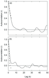 |
Figure 1 Examples of directional correlograms on the x-axis (solid line) and on the y-axis (broken line). Isotropy was assumed when both correlograms overlapped. (a) Isotropy; (b) anisotropy. Since transects were five 10-cm squares wide, the maximum lag in the correlogram following the y-axis direction was five (0.5 m). |
To estimate the effective sample size, we used the “model and Monte Carlo” procedure (Dale and Fortin, 2002) for two different kinds of models: the autoregressive model and the Markov model. Each model corresponded to a different approach in the kind of data used to fit the model: continuous data (from 0 to 1) in the autoregressive model and presence/absence data (0 and 1) in the Markov model. Continuous data were used to fit a second-order autoregressive (AR) model using the following equation:


Both models (AR and Markov) were fitted for each transect, and they were simulated 1000 times using a Monte Carlo approach to obtain artificial data. Restricted randomization was used in the simulation of the AR models (Fortin and Jacquez, 2000).
The resulting mean autocorrelation structure of the generated data was used to obtain the effective sample size, n′, to account for spatial autocorrelation, using the following equation:
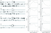 |
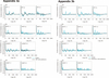
Figure 2 Cytisus cover and its associated spatial pattern (two-term local quadrat variance (TTLQV) and new local variance (NLV) as a function of scale) in transects 4 y after: (a) prescribed burning; (b) repeated prescribed burning; (c) wildfire in 20-year-old shrubs and (d) wildfire in 5-year-old shrubs. Since TTLQV and NLV values were similar between transects with the same treatment, results of only one selected transect per treatment are presented to facilitate interpretation. In Cytisus cover figures, black squares denote squares totally covered by Cytisus whereas white squares denote absence of Cytisus. The different gray fillings denote squares not totally occupied by Cytisus: from squares with high Cytisus surface occupation (dark gray) to squares with low Cytisus surface cover (light gray). |
Contrasts for the autoregressive (AR) and Markov models, including total initial and effective sample size calculated from each model, F values and significance. Mean cover difference (%) between contrasted treatments with a positive sign indicates that shrub cover was greater after the disturbance denoted with a (+) than the one with a (–) in the contrasts.
An ANOVA was used to test differences in Cytisus cover 4 y after the 4 different fire treatments: PF, RPF, 20 WF and 5 WF. We used the total effective sample size, resulting from the sum of the effective sample size either for AR or Markov models, for all transects. When the ANOVA was significant for a particular set of models, we used contrasts with the effective sample size for these models to test for differences in Cytisus cover 4 y after disturbance. We considered the following 4 contrasts: PF vs. RPF; 20 WF vs. 5 WF; PF vs. 5 WF; and RPF vs. 5 WF. The estimates of the contrasts were used to calculate the mean cover difference (%) between contrasted treatments (Crawley, 2007).
Spatial association in Cytisus cover was obtained by join count statistics (Fortin and Dale, 2005). Neighbourhoods were determined by rook moves (Fortin and Dale, 2005). We employed the three possible join count statistics for binary data which count the numbers of pairs of adjacent sampling units presenting the same category (JBB or JWW; B -black- for shrub presence and W -white- for shrub absence) or not (JBW) (Fortin and Dale, 2005). The statistics JBB and JWW assess the presence of positive spatial association, whereas the statistic JBW assesses the presence of negative spatial association. Instead of presence/absence data, the JBB join count was divided in three different categories (J22, J11 and J21), using continuous data. The 10 × 10 cm square with a 50% or higher Cytisus surface occupation was coded as 2, whereas the square with less than 50% Cytisus surface cover was coded as 1. We calculated the join count statistics J22, J11 and J21, where JBB = J22 + J11 + J21.
The spatial pattern of Cytisus was analysed using both the scale of pattern and the size of shrub patches. The scale of shrub cover in the different transects was analyzed using “Two term local quadrat variance” (TTLQV) (Hill, 1973). The variance in TTLQV is:
The average size of patches was assessed using “New Local Variance” (NLV) (Galiano, 1982). The variance in NLV is:  This method detects the average size of the smaller phase of the pattern (gap or patch) (Dale, 1999). In our case, since Cytisus cover was smaller than gap cover in all transects, NLV detected Cytisus average patch size in each transect. We used both TTLQV and NLV values to compare scale of pattern and average patch size respectively, between the different treatments.
The spatial pattern analysis was performed with the spatial statistics program PASSaGE v2 (Rosenberg, 2008). The rest of the analysis and simulations were performed using R (R Development Core Team, 2007).
3. RESULTS
Four years after fire, Cytisus cover in the transects ranged from 5% to 26% (Tab. I and Fig. 2). For both AR models and Markov models, after correcting for the effective sample size (App. 21), ANOVA and all contrasts were still highly significant (all, p < 0.001) (Tab. II). The contrasts indicated that, 4 y after the same wildfire, Cytisus cover in the at least 20-year-old stands (20 WF) was about 14% higher than in the 5 year-old stands managed by an earlier prescribed burning (5 WF). Four years after a prescribed burning (PF), Cytisus cover was about 10% higher than that found after a repeated prescribed burning in the same transects (RPF). Two additional contrasts, considering only transects with the same burnt shrub age, indicated small differences in mean shrub cover between PF and WF transects (6.4%), and very slight differences between RPF and WF transects (2.4%).
Correlograms for data and for AR model simulations showed that the second-order AR models generally maintained some kind of cyclic pattern after simulation because there was alternation between positive and negative autocorrelation values in the simulated correlograms (App. 3a1). In contrast, first-order Markov model simulations did not detect any kind of cyclic pattern (App. 3b1). Spatial association in Cytisus cover was obtained by join count statistics. The observed join counts for the statistics assessing both positive spatial association (shrub presence: presence - JBB- in all considered categories (J22, J11, J21) and shrub absence: absence - Jww-) were always higher than the expected values (App. 41). The join count JWB that assesses negative spatial association was also significant in all transects. As a result, Cytisus cover showed a patchy pattern in every transect.
The shrub cover after the different disturbances presented similar scales of pattern (Fig. 2). Thus, peaks in the TTLQV variance plots corresponded to similar values at block size (scale) in the PF, RPF, 20 WF and 5 WF transects, with peaks between 8 and 9 (0.8–0.9 m) (Fig. 2). In contrast, peaks in the NLV variance indicated larger block size (scale) values in PF transects (values close to 10 (1 m)) than in RPF, 5WF and 20WF transects (values close to 5 (0.5 m); Fig. 2).
4. DISCUSSION
Wildfires and prescribed burnings are likely to affect vegetation recovery in a different manner. In our study, both Cytisus cover and its spatial pattern 4 y after fire varied according to the disturbance type.
4.1. Cytisus cover after different fire disturbances
After accounting for the presence of spatial autocorrelation, shrub cover was found to be almost 10% greater after prescribed burning than after repeated prescribed burning on the same plots 4 y later. Thus, despite the important role of repeated fires in the spread of Cytisus (Debussche et al., 1980) and contrary to our expectations, a burning frequency of once every 4 y did not seem to increase Cytisus cover. However, it is necessary to be cautious with this conclusion because it emerges from a comparison between two quite similar treatments, since both prescribed burning and repeated prescribed burning transects were managed by a prescribed burning applied in the early 1990s. Contradictory results concerning the effect of fire frequency on shrub expansion have previously been reported. In general, fire suppression is the primary cause of shrub expansion in many grassland ecosystems. However, in C4-dominated grasslands of central North America, shrub cover increases with a fire frequency of once every 4 y (Heisler et al. 2003), which is similar to the fire frequency in our study. In contrast, as in our study, repeated burning was reported to reduce cover for other shrub species in an African savanna (Roques et al., 2001).
In general, fire intensity induces variations in the regeneration response (Knox and Clarke, 2006). Although the real fire behaviour was unknown, fire intensity was presumably higher in the 20 WF burnt plots than in the 5 WF ones, mainly due to differences in fuel accumulation. However, contrary to our expectations, Cytisus cover 4 y after wildfire was almost 14% greater in 20 WF transects than in 5 WF transects. As the 5 WF plots were being managed by an earlier prescribed burning, the lower cover in 5 WF actually suggests that fire frequency may have a greater influence on Cytisus recovery than fire intensity. Moreover, since resprouting vigor and post-fire survival have been related to the pre-fire size of the individual (González et al., 2007; Lloret and López-Soria, 1993; Moreno and Oechel, 1993; Quevedo et al., 2007), shrub age before disturbance may also contribute to the observed differences in shrub cover between the 20 WF and 5 WF transects. Assuming a higher fire intensity in wildfires (occurring in summer) than in prescribed burnings (in winter), the slight cover differences indicated by contrasts between PF or RPF and 5 WF (6.4% and 2.4%, respectively) also point to a low impact of different fire intensities or fire season on Cytisus regrowth.
We corrected for spatial autocorrelation but the effective sample sizes were still large so that small differences in shrub cover were statistically significant, although perhaps not biologically important (Morrison, 2007). However, correcting for spatial autocorrelation ensures that the statistical significance is legitimate, even if the differences between treatments are small.
4.2. Cytisus spatial pattern after different fire disturbances
Cytisus shrub cover had a patchy structure after fire disturbance as indicated by both join count statistics and correlograms for real data. As cyclic patterns present both positive and negative spatial autocorrelation, a crucial point for their application to ecological data is that the negative autocorrelation introduced may require inflation of the test statistic rather than deflation (Dale and Fortin, 2002). In fact, the test statistic required inflation (n′ > 1000) in four transects, all affected by wildfire (App. 2). This may indicate that fire severity or the processes (e.g., competition, available resources, etc.) that limit shrub regeneration may be stronger after a wildfire than after a prescribed burning or repeated prescribed burnings. However, not all the transects affected by wildfire required inflation of the test statistic and, therefore, we must be cautious with these conclusions.
Even though methodology is not the main concern of this paper, a relevant point in our approach is the study of spatial structures. Some years ago, Legendre (1993) pointed out that studying spatial structures was both a requirement and a challenge for ecologists who deal with spatially distributed data. Several years later, we find that although ecologists have used Markov models extensively for this purpose (e.g., Dale et al., 1993; Mark and Wilson, 2005), they have seldom used AR models (Lichstein et al., 2002), partly because of the mathematically complex implementation of autoregressive models (Cressie, 1993). In our study the amount of variation explained with the AR models was high, with adjR 2ranging from 0.51 to 0.79. This high amount of explained variation is usual when spatial structure is incorporated into models of ecological systems (Legendre, 1993).
It is generally agreed that TTLQV is one of the recommended techniques for pattern analysis (Lepš, 1990) and it has been used previously to describe spatial pattern in shrubs after a particular disturbance (Dale and Zbigniewicz, 1997). It should be noted that TTLQV is mathematically identical to wavelet analysis using the Haar wavelet and 3TLQV is identical to the use of the “French Top Hat” wavelet (Dale and Mah, 1998; Fortin and Dale, 2005). For either approach, local scores with positions along the transects can be calculated individually and mapped if that is desirable for the analysis. The scale of pattern in transects affected by different treatments was very similar (0.8–0.9 m), indicating that the different fire perturbations did not impact on the distance between the centres of neighbouring shrub patches. In contrast, the average size of shrub patches assessed with NLV may indicate that, 4 y after disturbance, repeated prescribed fires and wildfires reduced shrub patch size by half in comparison with prescribed burning (0.5 m vs. 1 m mean patch size). Overall, our results suggest that the scale of pattern is very stable in these communities despite being affected by different fire disturbances, whereas, in contrast, patch size may be more sensitive to different fire disturbances.
5. CONCLUDING REMARKS
From the management point of view, these results suggest that the effects of repeated prescribed burning were similar to those of a wildfire in reducing Cytisus cover and shrub patch size and, in consequence, that repeating precribed burning every four o five years may be an effective tool for reducing Cytisus cover. The decrease in shrub patch size after repeated prescribed burning may have relevant implications for habitat occupancy by birds (Pons et al., 2003) as well as for grassland productivity or plant biodiversity (Rigolot et al., 2002). However, repeating burning may have a negative effect on other key ecosystem processes (e.g., soil carbon storage or nitrogen availability).
In summary, the use of spatial analysis techniques may help to decide the best management option to achieve the desired ecosystem structure. Additional research is required to determine the importance of fire intensity and fire season in the spatial pattern of Cytisus regeneration after fire although our study indicates that they are less important than factors such as perturbation frequency and shrub age before disturbance.
Acknowledgments
J.M. Blanco provided statistical help. E. Marks improved early manuscript drafts. FM had a grant for a stay at the University of Alberta (2006 BE-2 00272) as well as a Ph.D. fellowship (2005FI 00801) from DURSI-Generalitat de Catalunya and the European Social Fund. Additional support came from the Spanish Ministerio de Agricultura (INIA, Balangeis, SUM 2006-00030-CO2-00) and the Spanish Ministerio de Educación y Ciencia (VULCA, CGL2005-08133-CO3).
References
- Campbell J.E., Franklin S.B., Gibson D.J., and Newman J.A., 1998. Permutation of two-term local quadrat variance analysis: general concepts for interpretation of peaks. J. Veg. Sci. 9: 41–44 [CrossRef].
- Chapin F.S.III, Matson P.A., and Mooney H.A., 2002. Principles of terrestrial ecosystem ecology, Springer, New York.
- Crawley M.J., 2007. The R book, Wiley, New York.
- Cressie N.A.C., 1993. Statistics for spatial data. Wiley series in probability and mathematical statistics, Wiley, New York.
- Dale M.R.T., 1999. Spatial pattern analysis in plant ecology, Cambridge University Press.
- Dale M.R.T. and Fortin M.-J., 2002. Spatial autocorrelation and statistical tests in ecology. Ecoscience 9: 162–167.
- Dale M.R.T., Henry G.H.R., and Young C., 1993. Markov models of spatial dependence in vegetation. Coenoses 8: 21–24.
- Dale M.R.T. and Mah, M., 1998. The use of wavelets for spatial pattern analysis in ecology. J. Veg. Sci. 9 :805–814.
- Dale M.R.T. and Zbigniewicz M.W., 1997. Spatial pattern in boreal shrub communities: effects of a peak in herbivore density. Can. J. Bot. 75: 1342–1348.
- Debussche M., Escarré J., and Lepart J., 1980. Changes in mediterranean shrub communities with Cytisus purgans and Genista scorpius. Vegetatio 43: 73–82 [CrossRef].
- Etienne M., 1989. Non destructive methods for evaluating shrub biomass: A review. Acta Oecol. 10: 115–128.
- Fortin M.-J. and Dale M.R.T., 2005. Spatial analysis. A guide for ecologists, Cambridge University Press.
- Fortin M.-J. and Jacquez G.M., 2000. Randomization tests and spatially autocorrelated data. Bull. Ecol. Soc. Am. 81: 201–205.
- Galiano E.F., 1982. Détection et mesure de l'hétérogénéité spatiale des espèces dans les pâturages. Acta Oecol. 3: 269–278.
- González J.R., Trasobares A., Palahí M., and Pukkala T., 2007. Predicting stand damage and tree survival in burned forests in Catalonia (North-East Spain). Ann. For. Sci. 64: 733–742 [CrossRef] [EDP Sciences].
- Heisler J.L., Briggs J.M., and Knapp A.K., 2003. Long-term patterns of shrub expansion in a C4-dominated grassland: fire frequency, and the dynamics of shrub cover and abundance. Am. J. Bot. 90: 423–428 [CrossRef].
- Hill M.O., 1973. The intensity of spatial pattern in plant communities. J. Ecol. 61: 225–235 [CrossRef].
- Kent M. and Coker P., 1992. Vegetation description and analysis, Boca Raton, FL, CRC press.
- Knox K.J.E. and Clarke P.J., 2006. Fire season and intensity affect shrub recruitment in temperate sclerophyllous woodlands. Oecologia 149: 730–739 [PubMed] [CrossRef].
- Legendre P., 1993. Spatial autocorrelation: trouble or new paradigm? Ecology 74: 1659–1673.
- Legendre P. and Fortin M.-J., 1989. Spatial pattern and ecological analysis. Vegetatio 80: 107–138 [CrossRef].
- Legendre P. and Legendre L., 1998. Numerical ecology. 2nd English ed., Elsevier, Amsterdam.
- Lepš J., 1990. Comparison of transect methods for the analysis of spatial pattern. In: Cornack R.M. and Ord J.K. (Ed.), Spatial processes in plant communities, Fairland: International Co-operative Publishing House, pp. 289–303.
- Lichstein J.W., Simons T.R., Shriner S.A., and Franzreb K.E., 2002. Spatial autocorrelation and autoregressive models in ecology. Ecol. Monogr. 72: 445–463.
- Lloret F. and López-Soria L., 1993. Resprouting of Erica multiflora after experimental fire treatments. J. Veg. Sci. 4: 367–374 [CrossRef].
- Mark A.F. and Wilson J.B., 2005. Tempo and mode of vegetation dynamics over 50 years in a New Zealand alpine cushion/tussock community. J. Veg. Sci. 16: 227–236 [CrossRef].
- Molinillo M., Lasanta T., and García Ruíz J.M., 1997. Managing mountainous degraded landscapes after farmland abandonment in the central Spanish Pyrenees. Environ. Manag. 21: 587–598 [CrossRef].
- Montané F., Rovira P., and Casals P., 2007. Shrub encroachment into mesic mountain grasslands in the Iberian peninsula: effects of plant quality and temperature on soil C and N stocks. Global biogeochemical cycles 21, GB4016. DOI:10.1029/2006GB002853.
- Moreno J.M. and Oechel W.C., 1993. Demography of Adenostoma fasciculatum after fires of different intensities in Southern California Chaparral. Oecologia 96: 95–101 [CrossRef].
- Morrison L.W., 2007. Assessing the reliability of ecological monitoring data: power analysis and alternative approaches. Nat. Areas J. 27: 83–91 [CrossRef].
- Økland R.H., 2007. Wise use of statistical tools in ecological field studies. Folia Geobot. 42: 123–140 [CrossRef].
- Pickett S.T.A. and White P.S., 1985. The ecology of natural disturbance and patch dynamics, academic press, New York.
- Pons P., Lambert B., Rigolot E., and Prodon R., 2003. The effects of grassland management using fire on habitat occupancy and conservation of birds in a mosaic landscape. Biodivers. Conserv. 12: 1843–1860 [CrossRef].
- Quevedo L., Rodrigo A., and Espelta J.M., 2007. Post-fire resprouting ability of 15 non-dominant shrub and tree species in Mediterranean areas of NE Spain. Ann. For. Sci. 64: 883–890 [CrossRef] [EDP Sciences].
- R Development Core Team, 2007. R: A language and environment for statistical computing. R foundation for statistical computing, Vienna, Austria, http://www.R-project.org.
- Ramsay P.M. and Fotherby RM., 2007. Implications of the spatial pattern of Vigur's Eyebright (Euphrasia vigursii) for heathland management. Basic Appl. Ecol. 8: 242–251 [CrossRef].
- Rigolot E., Lambert B., Pons P., and Prodon R., 2002. Management of a mountain rangeland combining periodic prescribed burnings with grazing: impact on vegetation. In: Trabaud L. and Prodon R. (Eds), fire and biological processes, Backhuys publishers, Leiden, The Netherlands, pp. 325–337.
- Roques K.G., O'Connor T.G., and Watkinson A.R., 2001. Dynamics of shrub encroachment in an African savanna: relative influences of fire, herbivory, rainfall and density dependence. J. Appl. Ecol. 38: 268–280 [CrossRef].
- Rosenberg M.S., 2008. Passage. Pattern analysis, spatial statistics, and geographic exegesis, Version 2. http://www.passagesoftware.net.
- Roura-Pascual N., Pons P., Etienne M., and Lambert B., 2005. Transformation of a rural landscape in the Eastern Pyrennes between 1953 and 2000. Mt. Res. Dev. 25: 252–261 [CrossRef].
Online material
 |
Appendix 1 Plot managed by prescribed burning on the Railleu study site. |
Parameters and adjusted-R2 for AR models and effective sample size (n′) calculated from both AR and Markov models. All AR models were highly significant (p-value < 0.001). Model parameters significance was indicated by: (***) p < 0.001; (**) p < 0.01; (*) p < 0.05; (n.s.) p > 0.05. Initial sample size (n) was 1000 in all the transects.
 |
Appendix 3 Correlograms for real data and AR model simulations for each transect (3a) and correlograms for real data and Markov model simulations for each transect (3b). For both figures: (a) prescribed burning; (b) repeated prescribed burning; (c) wildfire in 20-year-old shrubs and (d) wildfire in 5-year-old shrubs. |
Join count statistics for each transect (JBB, JWW and JWB, JBB was divided in three categories: J22, J21 and J11). The expected (Exp) and observed (Obs) values are based on rook moves. Join count statistics are significant when z values > | − 1.96| . Z values are indicated in parentheses below each observed value.
All Tables
Fire disturbance characteristics and Cytisus cover 4 y after disturbance in the 10 transects. Cover for repeated prescribed burning (RPF) and prescribed burning (PF) treatments was recorded in the same permanent transects.
Contrasts for the autoregressive (AR) and Markov models, including total initial and effective sample size calculated from each model, F values and significance. Mean cover difference (%) between contrasted treatments with a positive sign indicates that shrub cover was greater after the disturbance denoted with a (+) than the one with a (–) in the contrasts.
Parameters and adjusted-R2 for AR models and effective sample size (n′) calculated from both AR and Markov models. All AR models were highly significant (p-value < 0.001). Model parameters significance was indicated by: (***) p < 0.001; (**) p < 0.01; (*) p < 0.05; (n.s.) p > 0.05. Initial sample size (n) was 1000 in all the transects.
Join count statistics for each transect (JBB, JWW and JWB, JBB was divided in three categories: J22, J21 and J11). The expected (Exp) and observed (Obs) values are based on rook moves. Join count statistics are significant when z values > | − 1.96| . Z values are indicated in parentheses below each observed value.
All Figures
|
Figure 1 Examples of directional correlograms on the x-axis (solid line) and on the y-axis (broken line). Isotropy was assumed when both correlograms overlapped. (a) Isotropy; (b) anisotropy. Since transects were five 10-cm squares wide, the maximum lag in the correlogram following the y-axis direction was five (0.5 m). |
| In the text | |
|
Figure 2 Cytisus cover and its associated spatial pattern (two-term local quadrat variance (TTLQV) and new local variance (NLV) as a function of scale) in transects 4 y after: (a) prescribed burning; (b) repeated prescribed burning; (c) wildfire in 20-year-old shrubs and (d) wildfire in 5-year-old shrubs. Since TTLQV and NLV values were similar between transects with the same treatment, results of only one selected transect per treatment are presented to facilitate interpretation. In Cytisus cover figures, black squares denote squares totally covered by Cytisus whereas white squares denote absence of Cytisus. The different gray fillings denote squares not totally occupied by Cytisus: from squares with high Cytisus surface occupation (dark gray) to squares with low Cytisus surface cover (light gray). |
| In the text | |
|
Appendix 1 Plot managed by prescribed burning on the Railleu study site. |
| In the text | |
|
Appendix 3 Correlograms for real data and AR model simulations for each transect (3a) and correlograms for real data and Markov model simulations for each transect (3b). For both figures: (a) prescribed burning; (b) repeated prescribed burning; (c) wildfire in 20-year-old shrubs and (d) wildfire in 5-year-old shrubs. |
| In the text | |